The
expression density lock was
coined by a certain research assistant during landmark
studies at
UCLA's Institute of Transportation and Traffic
Engineering in 1954. Traffic flow
analyses using primitive Monte
Carlo simulation
identified
various causes of traffic
viscosity, including marginal friction and
critical absorption volumes.
Fifteen years
later, in the 1970s, density lock,
which pertains to highways not
surface streets, became known by a
misnomer: gridlock.
Hey, where's the "grid"?
Everybody in the world has
suffered from the adverse effects of density lock on
roadway capacity and speed.
The work at UCLA resulted in the earliest
deployment of ramp
metering, which is now widely applied
to relieve highway congestion.
Let us explore another
concept, first proposed in 1954, for
preventing density lock?
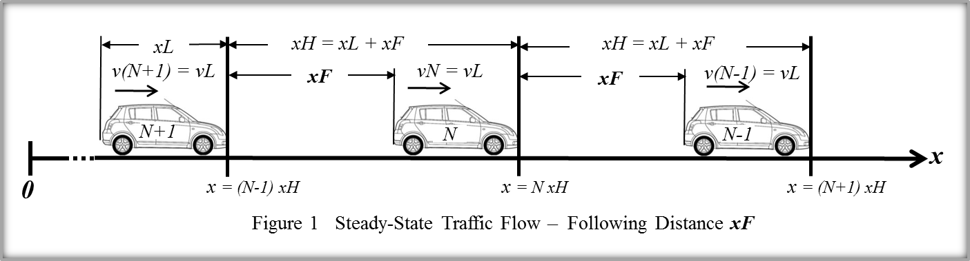
We begin with a generalized representation in Figure
1 of a vehicular
platoon operating in steady
state, which means traveling at a constant,
limited speed vL with a constant
following-distance between vehicles, measured from
bumper-to-bumper xF. The
instantaneous location of each vehicle along the x-axis
will be referenced herein to its front-bumper.
In
'congested flow', the speed of each vehicle is
constrained by the speed of the vehicle ahead, such that
vN ≤
v(N-1). The
following-distance xF is controlled
by the driver of the following vehicle.
Inasmuch as 40% of highway accidents involve
rear-end collisions, a 'safe' following distance,
often called a 'space cushion', needs
to be maintained, taking into consideration
roadway conditions and
visibility. The vernacular
expression 'tail-gating' is used to
describe the unsafe practice of following too
closely.
In Figure 1, the symbol xH
represents 'spatial headway', which is the sum of
the vehicle length xL and the
following-distance xF. For a
typical automobile, 12 ft < xL
< 15 ft. In the Density Lock puzzle, we
shall assume that xL = 13 ft.
Officially, the
term headway
refers to the timetH
required
for the passage of successive vehicles, and
tH
= xH / vL.
Modern driver-handbooks
recommend the "two-second
rule," such that tF ≥
2 sec, which would mean that tH
varies with vL according as tH
= 2 sec + xL / vL.
However,...
Your puzzle-master lives in
France, where he has observed stripes painted
alongside highways that mark one-second intervals
corresponding to the posted speed limit vL.
Pictorial signboards on the wayside provide
guidance to drivers for xF by
indicating that vehicle N should
leave an empty stripe behind any stripe ahead that
is occupied by vehicle N-1.
Observations of driving
behaviors on two continents suggest that an
estimate of tF= 1.5
seconds would be more realistic for use in
the Density Lock
puzzle.
As an illustration, consider a roadway in the U.S.
with a speed-limit vL = 35 mph (~50
ft/sec). To assure a safe following-distance using
tF= 1.5
sec, xF = 75 ft, which calls for xH
= 88 ft, and headway tH = 1.75 sec.
It may be worth noting that 'recommendations' in
mid-twentieth century driver-manuals often said, "allow
one car length for each 10 mph of speed." Back
then cars were longer, say, 15 feet, which suggests that
xF = 53 ft for 35 mph (22 ft closer),
and, since xH = 68 ft, the headway tH
= 1.4 sec.
Speed
= Flux / Density
Individual
users of transportation systems care mostly about Speed. They want to
get from where they are to where they want to be.
Faster the better. Speed is measured by
distance traveled per unit of time -- miles per
hour. In vehicular transportation, limits
are imposed by roadway conditions,
by neighborhoods such as residential areas
and business districts and school
zones, by weather and visibility -- oh, and
by traffic.
Managers of transportation systems care
mostly about traffic flow -- Flux.
More the better. The obvious objective of
'traffic managers' is to maximize the number of
vehicles moving through the system per unit of time --
vehicles per hour. Flux is limited to
various capacities within the infrastructure: by extra
lanes on roadways and ramps on highways, by
cross-streets and signals and stops -- oh, and by
traffic.
Traffic means congestion -- Density.
Congestion comes from demands on the system
exceeding 'free-flow' capacities. Density is
measured as the number of vehicles per unit of distance
-- vehicles per mile. Ironically, the objective
for traffic managers is not to minimize
density. Here's why. When roads and highways
are relatively empty, congestion may indeed be low, but
so is flow. Individual users will benefit with low
flow wherein speeds may be faster. For sure, speed
will be limited by something other than
traffic. Ah, but then there are fewer users being
served by the transportation system. Do traffic
managers actually worry when their capital-intensive
investments are under-utilized? Some do, maybe,
but not a lot.
The simple
expression vmi/hr
= qveh/hr
/ kveh/mi
offers us a rich set
of relationships. Solvers will benefit from
studying the fundamental
diagram of traffic flow, where they will learn
that for a given value for q, there are
two values for k and thus two values for
v, one in 'free-flow', the other in
'congested flow'. To test remedies for
Density Lock we must focus
on congested flow.
Speed = Flux
/ Density
Management
in Congested Flow
Speed
of each vehicle N is
limited by the speed of vehicle N-1
immediately ahead. Flux
through a system is framed by traffic
management via designs and regulations.
Density
is absolutely controlled by the individual
drivers in vehicles!
Sophisticated solvers will take note of the
exclamation point.
Below is a graph of the three
traffic variables...
...on a section of highway. The green dots
● in
the graph show that in congested flow, a platoon
of vehicles traveling at60 mph
will be limited to a maximum density of 33
veh/mi which imposes a limit of 2,113 veh/hr per
lane maximum flux in that section.
During 'rush hour', the density
of vehicles in the section of highway will
necessarily increase as vehicles enter the lane on
ramps from side-roads and other highways. The
graph shows that when the traffic density in that
section of highway doubles to 66 veh/mi, the maximum
flux, which is the carrying capacity of the
lane, will be slightly reduced to 2,003 veh/hr, but
the maximum speed of individual vehicles will be
decreased 50% -- implying twice the trip-time.
Exclamatory punctuation is invited.
We
consider now two transient-states in congested flow,
beginning with the inevitable need for vehicles to slow
down or to stop. Stops occur in various
forms. Three come readily to mind...
Emergency Stops can occur in any
lane on any roadway. Whereas in congested
flow, a sudden slow-down can produce a traffic
'jam', depending on density, but in 'free-flow', not
so much. A 'platoon' can form behind the
stopped vehicle, its length determined by the
duration of the stop. Release of the jam is
generally an ad hoc proposition.
Boulevard Stops
require all vehicles in each lane to come to rest or
to queue up at an intersection and wait for one
vehicle of cross-traffic, if any. Subsequent
vehicles in the lane, if any, creep forward and wait
their turn, first-come-first-served,
then start up one-by-one, with releases being
self-regulated and acceleration generally in
'free-flow'.
Signalized Intersections, wherein
vehicles are regulated for stopping and releasing by
automatic controls, often synchronized among groups
of intersections, apportioned by traffic detection
that make 'calls' for lane-control and for
coordination with pedestrians. In congested
flow, signals intentionally create traffic 'jams'
along with 'platooning'.
For exemplifying transient-states in congested flow,
we shall use the Signalized
Intersection.
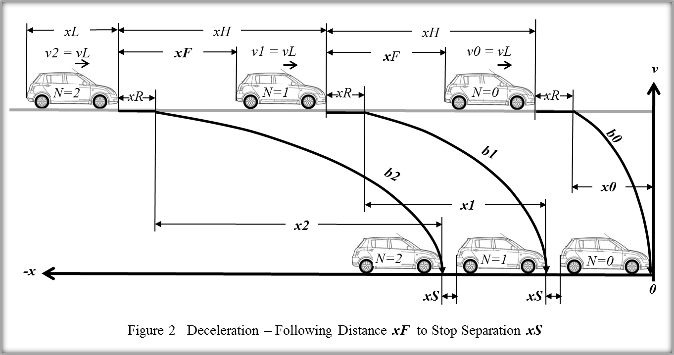
Figure 2 applies a tool known as a phase-plane,
which plots the first derivative of a variable against
the variable.
In this case, vehicle speed v =
dx/dt
is
plotted on
the vertical axis against
linear dimensions on the horizontal axis x.
Events referenced to time cannot be
depicted on a phase-plane plot. Instead, two
'snap-shots' are superimposed in the diagram.
They represent [a] the point in space where the driver
of the first vehicle N=0 has observed a
yellow
aspect signal and has decided that the vehicle
can be brought to a safe stop at the intersection
before the red aspect appears and [b] any time after
all the vehicles in the platoon have been brought to a
stop.
Vehicles
are shown here being braked to a stop at a red signal.
This begins the formation of a platoon. The first
vehicle N=0 is assumed to be slowing at a
constant braking deceleration b0 reaching
v0 = 0 at location x = 0.
A constant deceleration appears as a
parabola on a phase-plane plot, inasmuch as braking
distance x0 = vL2 /
(2 b0). A
'reaction' distance xR is shown as
the same for all vehicles in the platoon. It
is an estimate for the distance traveled at vL
during tR, commonly called
'reaction time' in most jurisdictions.
Signals in the U.S. are typically located on the
far side of the intersection, such that drivers in
some vehicles behind N=0 will be
able to see the light and plan their
deceleration. That interval tR
allows for [a] the 'perception' by each driver of
an existential need to decelerate based on
conditions ahead and [b] the 'mode-change delay'
from propulsion to braking.
For the base case in the Density
Lock puzzle, we will let tR = 0.75
sec.
The total stopping distance can be
generalized for each vehicle in the
platoon in the following
expression vL tR + vL2
/ (2 bN).
Figure 2 shows common following-distance xF
between vehicles moving at vL, which was
introduced in Figure 1 above. Introduced in Figure
2 is a typical separation distance xS
between stopped vehicles. Most drivers allow 1 ft
< xS < 3 ft. For the base
case in the Density Lock
puzzle, we shall use xS = 2 ft.
An emergency stop on a highway might let
vL = 60 mph (88 fps), and xF
= 132 ft. Nota bene, each 'space
cushion' will get 'squeezed' from xF =
132 ft to xS = 2 ft. With xF
> xS, the allowable braking
distances cumulatively increase for successive
vehicles in the platoon, and xN > x(N-1),
assuring the safety of bN < b(N-1).
With elementary algebra, one finds that xN =
x0 + N (xH - xS - xL). Notice that xN
does not vary with tR, inasmuch as xR
is nested within both xF and xH. To ascertain
the required deceleration for each vehicle, we writevL2
/ 2bN = vL2
/ 2b0 + N (xH - xS - xL)
and solve for bN as a function of b0.Thus bN = b0 vL2
/ [vL2
+ 2N(xF - xS)
b0].
As we see here, traffic density sure does increase
when vehicles in a platoon slow down...
...thus in stopping from 60 mph, density goes from 33
veh/mi to 352 veh/mi, a
ratio of ~11:1.
The most extreme congestion is called a 'jam' by
traffic managers. Vehicles within a jam are prohibited
by density lock from
moving much. Solvers will be invited to evaluate a
counter-intuitive proposal for relieving traffic
jams. But first we need to consider the realities
that arise during another transient-state in vehicular
flow. Figure 3 applies a phase-plane to help us
understand what takes place in a platoon of vehicles
recovering from a traffic jam.
The
leading three vehicles in a platoon are shown
stopped at a red light, with
the first vehicle, N=0, at
location x = 0. They are
separated by bumper-to-bumper distances xS.
As the light turns green, the first vehicle N=0
is the only vehicle in the whole platoon
that is not jammed but free to begin its
acceleration a0 straight away,
limited only by roadway conditions ahead.
All the rest of the vehicles in the platoon are
operating in congested flow, with separations
constrained to increase gradually from xS
toward xF. For
modeling the typical profile for vehicles N
= 1, 2,... three alternative concepts
come to mind...
[1] Postulate a waiting time tW,
and each vehicle N is assumed
to remain stopped after the start-up of
vehicle N-1 before beginning
its own acceleration; however...
[2] An interesting model for driving behavior
would allow eachvehicle to start-up at will and
accelerate gradually one-by-one to facilitate
the build-up of space between
vehicles. Such is the driving behavior
modeled in Figure 3 above; however...
[3] That research assistant at UCLA, now an
octogenarian living in France, has come to
realized that the most reasonable model would
have each vehicle N creep
forward to the entrance of the intersection as
allowed by the instantaneous location of
vehicle N-1 ahead. The creep-to-the-stop-line
concept will be brought into consideration on
the solution page of the Density Lock puzzle.
The first vehicle is
shown accelerating at a0 in
'free-flow' to the limiting speed vL
over a distance of x0 = vL2
/ (2 a0), thence to
continue at vL. Vehicle N=1
begins accelerating at about the same time,
but its acceleration a1 < a0.
The two
profiles appear to cross each other at a point
P beyond location x = 0.
No reason to get alarmed by that, though...
Keeping in
mind that the phase-plane plot is not
correlated in time, we realize that the
common point P is reached at
different times for the two vehicle.
Same for other vehicles in the platoon as
they start up and follow along behind.
They each reach some intermediate speed vP
at about the same location xP.
Sophisticated solvers may enjoy the
challenge of finding the location of xP
and the value of vP. Or
not.
Acceleration a1 will be
modeled as chosen intuitively by the
driver of vehicle N=1 -- chosen
so as to reach vL at a point
along the roadway behind vehicle N=0
by the headway distance xH,
where xH = xF + xL. Kind
of astonishing, when you think about it, that
such an outcome can be assured by
instuition. Likewise, vehicle N=2
accelerates at a2 so as to
reach vL at a distance xH
behind vehicle N=1, and so
forth. One can generalize the
acceleration distances as xN = vL2
/ (2 aN).
Each vehicle reaches vL
at the location which satisfies the following
equation: xN = x0 + N (xH
+ xS + xL), which can be expanded
to read vL2
/2aN) = vL2
/ 2a0 + N
(xH + xS + xL) and solved for
aN as a function of a0.
Thus, aN
=a0 vL2
/ [vL2
+2 N (xF - xS) a0].
Sophisticated
solvers will not be surprised to see that the
expressions for aN and bN
are identical. It is merely a
consequence of symmetry in the model
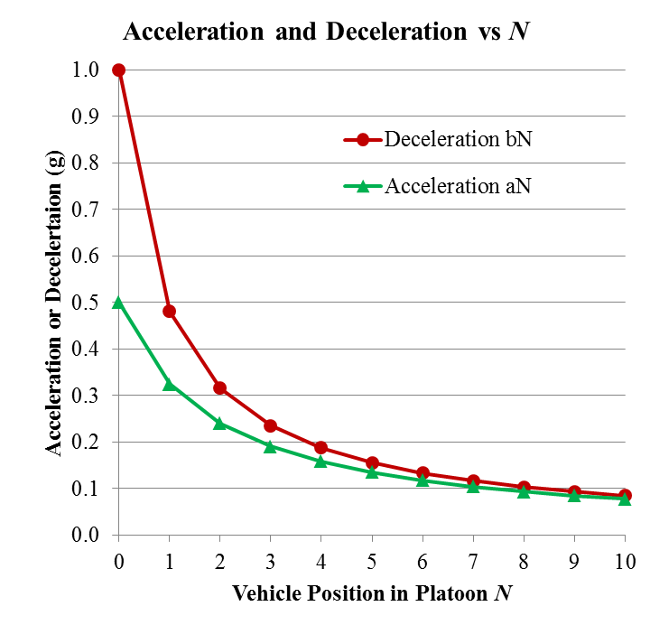
formulation. Here is a
graph showing how aN and bN
decrease with N in the
illustration above with vL = 35
mph. The value of b0
was selected to represent a case of an extreme
deceleration -- 1 g, the limit that can be
achieved with four-wheel braking and unity
coefficient of friction between rubber and
roadway surface. The chosen value of a0
= b0 / 2, and produces a a curve
that might reasonably characterizes the
behavior of vehicles when the light changing
from red to green.
Dean's
Award for 1955
As
mentioned in the introduction to the puzzle, 60 years ago a
certain research assistant at UCLA's Institute of
Transportation and Traffic Engineering made a
radical proposal to the world in the
form of a question...
Would
mandating
that vehicles stop at prescribed
separations prevent density
lock?
He obtained sponsorship
from renowned traffic expert Dan
Gerlough and conducted an experiment
to find out. Ten fellow undergraduates
in UCLA's College of Engineering gave up a
Saturday morning to drive their cars around
the campus on a blocked off street, where a
temporary traffic signal had been set
up. Each driver was assigned a number
and given a 'script'. They assembled
in a parking lot to be randomized.
They then drove as a platoon onto the street
and stopped under the control of the
signal. Every car had a prescribed
stopping location. Ten runs were
conducted for each of two configurations.
The base case
prescribed xS = 2 ft.
The experiment case prescribed xS
= xF / 2.
The stop-locations were marked with
numbered traffic cones. As
the light was switched to green, the drivers
accelerated to vL = 35 mi/hr.
At several places along the roadway
were pairs of vehicle detectors, each pair
separated by 3 ft to ascertain speeds.
Signals from the detectors were charted on a
roll of paper, to be analyzed in timing
measurements. The resulting
thesis won the dean's award for 1955.
Solvers can decide if that honor was
deserved.
 The
expression density lock was
coined by a certain research assistant during landmark
studies at
UCLA's Institute of Transportation and Traffic
Engineering in 1954. Traffic flow
analyses using primitive Monte
Carlo simulation
identified
The
expression density lock was
coined by a certain research assistant during landmark
studies at
UCLA's Institute of Transportation and Traffic
Engineering in 1954. Traffic flow
analyses using primitive Monte
Carlo simulation
identified